One of the prevailing terms bantered around in the zeitgeist of modern society is “artificial intelligence," or AI. While artificial intelligence infers the imminent rise of sentient machines, and robots taking over the world, in reality this is far from the truth. For most, the AI of today turns out to be a “smart speaker” that will play music and turn on your porch light --- well, after you ask three times (alexa … aleXA? … ALEXA!).
Needless to say, artificial intelligence is mostly a term used in marketing and entertainment.
However, today we are seeing amazing results with foundational computer interactions – speech recognition is making unparalleled accuracy gains, computer vision systems are able to recognize objects in real time and recommendation systems are becoming uncannily accurate. These gains are the result of a set of smart algorithms that all under the title “machine learning.”
Finding Things
Machine learning is a broad term, used to describe a set of algorithms that do nothing more that identify data.
- Is this a picture of a cow or a pig?
- Is this data value greater that 12?
- Was the word "Alexa" spoken?
This identification process is referred to as “data classification” (or just “classification”), and machine learning is just a group of classification algorithms used to identify data.
Simple Classification – Finding the Color Red
In its simplest form, data classification is nothing more than a straightforward mathematical statement able to identify information based on some property of the source data.
A great example of this is in the identification of color. In standard computer imagery, color is represented as three components: red, green, blue or RGB. Normally the RGB components are represented as a byte (8 bits of data), with a data range of 0 to 255.
The identification of a specific color is nothing more than a simple test of equality. For example, to determine if a color is red, the equation (in a simple pseudo code) is nothing more than:
If color.Red == 255 and color.Green == 0 and color.Blue == 0 then
    Print “The color is RED!”
To show this working, let’s apply this “red color” classifier to each pixel in the following image:

Figure 1: Spark Lounge
Setting all non-red pixels to black, we get the following image:

Figure 2: Sorry - pure red pixels don’t exist in the wild.
The results are black – how did this happen? Turns out, no pixels of pure red (RGB value of (255, 0, 0)) were in the image. The visibly red sections have RGB values that are red dominant, but not a pure red color value.
If we loosen the parameters in our color filter so that the cutoff for a red value is the following:
If color.Red > 150 and color.Green  < 100 and color.Blue < 100 then
    Print “The color is mostly RED!”
We get the following result:

Figure 3: Mostly red areas
This is a result one would expect when identifying the red pixels in an image, and demonstrates that what appeared to be a simple classification effort needed a little adjustment to get the expected results.
Useful Color Classification
While finding red areas in an image isn’t that useful, pixel color-based algorithms do have real-world applications. These algorithms are well known, fast and efficient. In applications with definitive results, this type of pixel-based classification technique provides a great solution.
A great example is the application of remote sensing imagery and agriculture. Just using color data that include infrared values, the health of a crop is easily determined. By applying a Normalized Difference Vegetation Index (NDVI) classification to image data, farmers and agriculture managers are able to gain valuable insight into crop health and better manage their resources to increase overall yields.
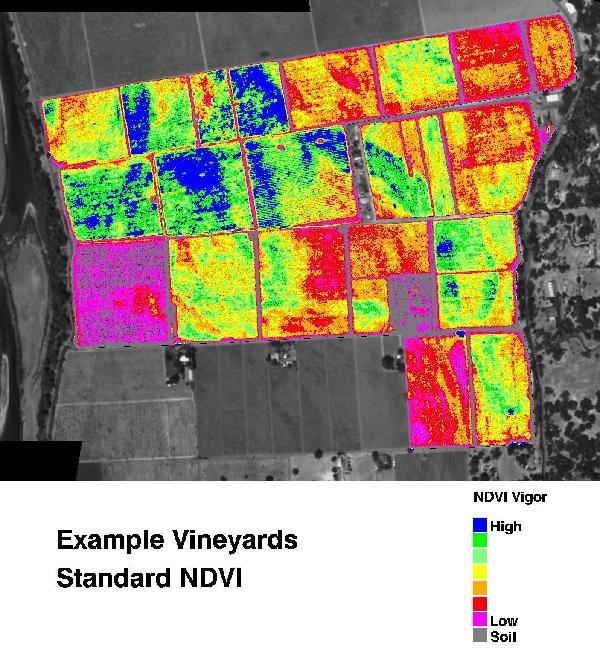
Figure 4: Crop health using pixel-based classification (NDVI)
The above picture shows the result of this type of classification on satellite imagery. With field areas clearly visible, the blue and green areas reflect healthy crop areas, while orange and red reflect areas that need attention.
How Do I Find a Red Chair?
Deterministic mathematical-based classification techniques are powerful, well understood and efficient. They provide a means to gain high-level insight into information content, and have proven valuable in solving real-world problems.
However, these solutions fail to scale and solve high-level classification needs. How could you identify a red chair – any red chair, from any angle? It’s almost impossible to break this type of object classification into a simple mathematical equation.
Classification of real-world, complex information often doesn’t follow simple mathematical exactness. Variability and dynamic complexities make this extremely difficult. But a method that learns from the information being classified, and adjusts for complexities and slight variabilities in information, could be successful in this form of data classification – this is the promise of machine learning.
Machine Learning
The approach machine learning algorithms use is to leverage data itself to refine the classification process. By using data values as part of the classification process, machine learning algorithms “learn” to identify values in complex data sets.
In the field of machine learning, classification algorithms are grouped into two broad categories: unsupervised and supervised classification. The breakdown between these two approaches is straight-forward: the use of example or training data. Unsupervised methods required no training or simple values, while supervised methods do.
Unsupervised Classification
The unsupervised classification technique requires no examples or training values as part of its processing. These algorithms have no prior knowledge before execution, and use the underlying values of the data being analyzed to perform the classification, looking for statically unique structures in the data and marking these as unique classes.
A common example of an unsupervised classification algorithm is data clustering. This algorithm finds adjacent data elements of similar values and “clusters” them together into classes. The resultant groups (clusters) contain objects that are more similar to each other than other objects in the data set.

Figure 5: Unsupervised classification using data clustering
While the results from unsupervised classification are often not as exact as supervised techniques, they provide a method to rapidly gain an overview of the underlying structure of a data set, which in turn helps guide further data evaluation and selection of analytical approach.
Supervised Classification
With a supervised classification methodology, training data is applied to the classification algorithm to teach the algorithm how to find the desired results. Training data might consist of a simple set of data points or involve thousands of images of a desired object. The key factor is that the data is identified or labeled with the expected results.
Using training data, as the classification algorithm is applied to the data, the results are compared to the expected values. If the results are incorrect, parameters within the algorithm are adjusted to correct the error. As the training progresses, the classification algorithm's settings are refined, eventually converging on values that actually perform the desired classification. Once training is completed, the algorithm settings and associated structure (often called a model) are packaged and deployed for classifying non-training data.
Finding Red
Earlier, we outlined the implementation and use of a simple, mathematical classifier to identify the color red. To accomplish a similar classification result using a supervised machine learning methodology, the following notional steps are used.
Selecting a Machine Learning Algorithm
A wide variety of machine learning algorithms/approaches exist. For this example, we’ll use our “SparkFun Flame Classifier” algorithm (yes, this is made up, but it helps convey the concepts).
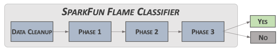
Figure 6: Classifier Structure
This classifier has several distinct stages, each feeding into the other stages with the final stage providing the classification results.
Training the Machine
To train the algorithm to provide the desired results, data that is identified as the desired results (as well as non-desired results) are used. In this case, since we are looking for the color red, a selection of red values and non-red values are applied to the algorithm.
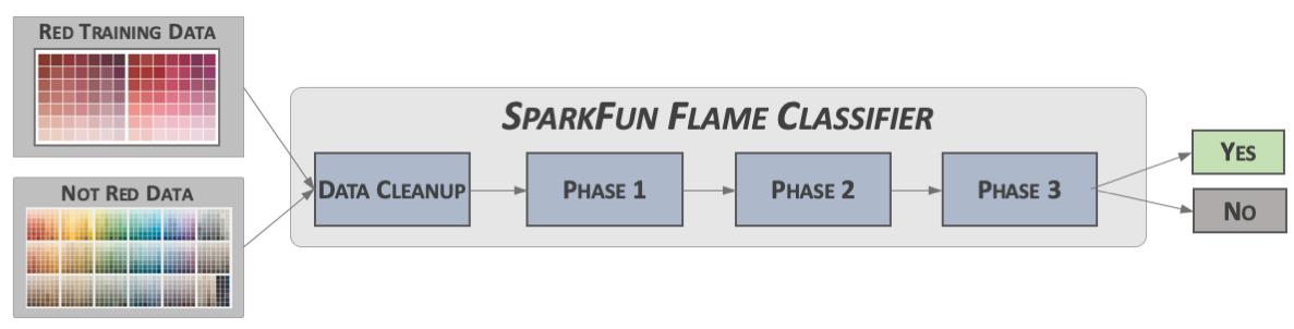
Figure 7: Training Concept
As training data is applied, the results are used to back-propagate values into the algorithm to adjust the overall model settings. The amount of adjustment applied depends on the algorithm, as well as whether the correct results were calculated.
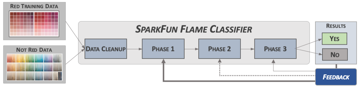
Figure 8: Training the Red Classifier
Using the Classifier
Once training is completed and the results validated, the results of the training session – the model – are placed in a deployable format and loaded into an operational setting.
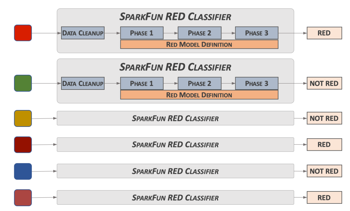
Figure 9: Running the Red Classifier
While just an example, the creation and training of this “Red Classifier” provides a great overview of the general machine learning development, training and deployment.
Neural Networks
The recent rapid increase and deployment of machine learning is centered around the use of a learning methodology called neural networks. These algorithms are inspired by the network of neurons within the human brain, using layers of information to transform nodes that are interconnected to form an overall network of information classification.
The layers of a typical neural network are simple in concept, but complex in reality. The structure is grouped into three general classifications: input layer, hidden layers and outputs. The general structure is outlined in the diagram below.
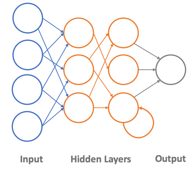
Figure 10: General Structure of a Neural Network
It’s worth noting that the outputs of each layer are not always connected to the inputs of the next layer. Additionally, the output of a node can be feedback into itself, allow the node to retain some “memory.” Overall, the structure and topology of the network is dependent on the function it’s performing.
Training
Like the simple classifier discussed earlier, neural networks are trained across a variety of inputs, using the results of the output layer to feedback into the settings of the nodes that make up the neural network. Using a similar back-propagation methodology as noted earlier, the training operation is performed across a wide set of training data to refine the capabilities of the neural network.
Training is a resource intensive process that requires extensive compute power and storage. Processing needs on the order of exaflops (a billion billion (1018) math operations) and terabytes of training data are often needed for modern neural networks used in speech and image recognition. Once training is completed, the resultant model is cleaned up (pruned) to eliminate non-used paths, and then serialized to a persistent data format and used in an operational setting to perform classification. This operational phase of a neural net is often called the process of inference.
Interference
The classification of data in the field is called inference. It is the process of “inferring” the results of a classification process. The results of this classification process are often given as a probability – a confidence value that the network believes a specific item/object is being identified.
While the process of inference uses significantly less compute resources when compared to the training phase, it still requires extensive local resources to deliver results in real-time.
To meet the requirements of inference, specialized hardware and software are being developed and deployed. NVIDIA and Google have both released computational hardware and software designed to live on the network edge – running on relatively low power while delivering real-time inference support.
Hardware
The great advancement in neural networks is the application of hardware to the network training process. The use of modern Graphics Processor Units (GPUs) – aka graphics cards – delivered incredible parallel processing capabilities. Specialized FPGAs also provided similar results, bypassing the CPU chokepoint to deliver exponential gains in neural network execution.
In addition to hardware gains, software and system architecture advances also enabled the rapid adoption of neural networks and machine learning. With the pairing of hardware-accelerated network execution and the resource aggregation and management capabilities of modern cloud computing platforms, machine learning not only became possible, its use exploded across the information-based systems and technology landscape.
Living on the Edge
The recent advances in machine learning have been on the “edge” – the far fringes of network computing. The devices and sensors that make up the “Internet of Things” – aka IoT – form the edge of the computing ecosystem. In the past, these sensors and devices were nothing more than data collectors – sending any information they detected to a larger system for processing and evaluation. Today, the processing and decision making are performed on these edge devices.
Recent developments from Google, NVIDIA and others have focused on the edge environment. Specialized hardware that offers signification performance while using minimal power are now available for use in standard packages that utilize familiar software environments.
The NVIDIA Jetson Nano Development Board and the Google Coral Development Board both deliver a Raspberry Pi-like platform with signification compute processing capabilities designed for neural net inference on the edge.
The big advancement is deployment of network inference capabilities within microcontroller environments. SparkFun was a leader in this effort and worked closely with Google to bring to the market one of the first, low-cost, high-performance microcontroller boards to the market.
Designed for audio processing, the SparkFun Edge Development Board delivers a low-power, low-cost solution to research and deployment of machine learning inference to the remote edges of the network.
When Will the Robots Take Over?
While the robot apocalypse has been promised for years and has reached a frenzied level recently, the truth is artificial intelligence is more hype than reality. However, smart machines are having a huge effect on our lives.
Major advances in classification technologies, and machine learning in particular, have incredible impact in our daily interactions. Computer speech recognition has reached exceptional accuracy, making machine-voice interactions commonplace. Machine image recognition and vision technologies are revolutionizing processes in factories, farms and even home security systems. And the advent of machine learning within the edge computing environment enables the continued proliferation of small compute devices within our environment.
Like other advances in low-power and embedded computing, SparkFun will continue to deliver the products, technologies and practical knowledge for edge computing. SparkFun's recent collaboration with Google on our Edge board is just the beginning of an effort to usher in machine learning and all the technologies it delivers into the edge of the computing universe.


Interesting overview! You said this fantastically.
Nicely done. Good overview. Thanks!